This is the second part of three blog posts regarding the work we have been doing at the city of Amsterdam, focusing on bias in machine learning. If you have made it this far after having read part 1, you should now have a decent understanding of some important concepts regarding bias in machine learning, and why it’s important to the municipality. Or perhaps you jumped straight here, because you already knew all that, in which case: good for you and welcome!
Recall that in these blog posts, we are concerned with making sure that different groups of people are treated fairly by our machine learning model when a suspicion of illegal holiday renting at their address arises. In part 1 we explained why this is important to the city of Amsterdam and dove into the theory around bias in machine learning. In part 2, we will start getting practical and look at the actual methodology we used. There is unfortunately not (yet) one perfect way to handle bias in machine learning, but hopefully, this example will inspire you and make it just a little bit easier to carry out a bias analysis yourself.
Context
Suppose that citizens are renting out their apartment to tourists. Since the city of Amsterdam suffers from a serious housing shortage, they are only allowed to rent out their apartment for a maximum of 30 nights per year, to at most 4 people at a time, and they must communicate it to the municipality. When a rental platform or a neighbor suspects that one of those requirements is not fulfilled, they can report the address to the municipality. The department of Surveillance & Enforcemen can then open a case to investigate it.
The subject of this blogpost is the machine learning model that supports the department of Surveillance & Enforcement in prioritizing cases, so that the limited enforcement capacity can be used efficiently. To this extent, the model estimates a probability of illegal holiday rental at an address.This information is added to the case and shown to the employee, along with the main factors driving the outputted probability. This helps to ensure that the human stays in the lead, because if the employee thinks the main drivers are nonsense, they will ignore the model’s advice.
At the same time, if they do start an investigation, it will help them to know what to pay attention to. A holistic look at the case (including the model’s output, but also the details of the case and requests from enforcers or other civil servants) then leads to the decision to pay the suspected citizen an investigative visit or not. After the investigation, supervisors and enforcers together judge whether there was indeed an illegal holiday rental or not. The purpose of the model is thus to support the department in prioritizing and selecting cases, while humans still do the research and make the decisions. It is good to note that in principle, all cases do eventually get investigated.
Methodology
Our goal is to analyze bias in the outcomes of the trained model, specifically: the probability of illegal holiday rental assigned to a case by the model. As we saw earlier, two sources of such bias are the data and the algorithm itself. This naturally leads to two ways of doing the analysis, namely by analyzing the data and/or the algorithm. A third option is to analyze bias in the outcomes. This is less complicated, because it is well-scoped and the outcomes are readily available on the train and test set. Since we're looking to investigate specifically the potential discriminatory effects of using the model in practice, and not those of the entire working process, this is the option we decided to go with. This does mean that it is not possible to exactly pinpoint the causes of a bias if we find one, although you can often make an educated guess about the ‘why’ in hindsight.
Having sorted that out, we come to the actual analysis, which can be divided roughly into 8 steps:
- Decide sensitive attributes to investigate
- Construct hypotheses about features causing indirect bias.
- Select metrics
- Analyze direct bias.
- Analyze indirect bias through underlying sensitive attributes.
- Analyze indirect bias through features.
- Evaluate results with stakeholders.
- Mitigate bias when necessary.
1. Decide sensitive attributes to investigate
To be able to do the analysis, we need to think about which attributes we do not want the model to discriminate on. For machine learning within the municipality, the following sensitive attributes can be considered relevant (in various degrees depending on the application):
- nationality
- country of birth
- gender
- sex
- sexual orientation
- religion
- age
- pregnancy
- civil status
- disability
- social class
- skin color
- ethnicity
- political views
- health
- genetics
We need information about these attributes to analyze them. However, not all of them are registered by the municipality or even by the government in general, in many cases for good reason. We mention the complete list here anyway to be aware of potential blind spots in the analysis. The attributes that were available within the municipality had never been used for the purpose of a bias analysis before. For that reason, we first defined the legal grounds on which this sensitive data could be processed .
2. Construct hypotheses about features causing indirect bias
As we know, some seemingly-innocent features may be correlated with a sensitive attribute, causing indirect bias. The second step in the analysis is to brainstorm about such relations. We systematically went through our list of features and were very liberal at this step: if we could come up with any logic why a feature could potentially cause indirect bias, we included it as a hypothesis. This resulted in a list of hypotheses about correlations between features and sensitive attributes.
3. Select metrics
We are not supposed to say that one step is more important than the others but selecting the metric(s) carefully is quite crucial. Bias is not a one-dimensional concept and multiple metrics are often needed to get a full overview.
We have already seen that individual fairness and group fairness are very different concepts, and within those two streams, there are still many more fine-grained metrics. At the same time, it is impossible to improve all metrics simultaneously. For that reason, we decided to look at a few metrics, and select one main metric to guide our decision-making in the analysis.
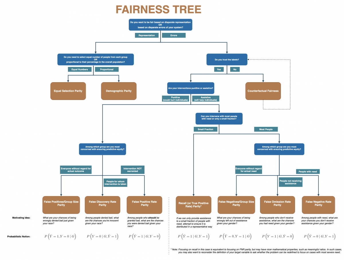
The “fairness tree” below was of great help in selecting the primary metric. Studying the metrics present and the ones not present in the tree helped to understand the implications of the choice better. Other helpful references were the documentation of AIF360 and Aequitas.

Fairness tree (Center for Data Science and Public Policy, University of Chicago)
Exploring the tree, we decided that:
- The model should be fair based on disparate errors, because of what we call ‘proportionality’ in municipality-speak: since investigations are a burden on a citizen, they should only be done when necessary.
- Although there is always a risk of false negatives when working in the domain of investigations and enforcement, in this case we generally trust the labels.
- Our interventions (investigations) are punitive.
- We’re most concerned with predictive equity among those addresses where an investigation was not warranted, again due to proportionality.
These considerations led us to the false-positive rate parity as the primary focus, implemented in the false-positive rate ratio. Many metrics can be looked at either as a difference or a ratio, but they convey the same information. In hindsight, it’s probably easier to use the difference. To understand this specific metric let’s look at the false-positive rate.
The false-positive rate (FPR) is calculated as the ratio between the number of negative events wrongly categorized as positive (false positives) and the total number of actual negative events (regardless of classification):
FPR = FP / N
So, what does false-positive rate parity mean for two citizens that get reported by their neighbor? If they’re both on the list of potential cases, but neither has an illegal holiday rental, then both should have the same probability of getting (wrongly) investigated.
The false-positive rate ratio (FPRR) is then defined as:
FPRR = FPRA / FPRB
Using the four-fifths rule (explained in the first blog post), it can be interpreted as follows: a FPRR
- between 0.8 and 1.25 is considered acceptable;
- lower than 0.8 means that group B is being discriminated;
- higher than 1.25 means that group A is being discriminated against.
A useful way to summarize the FPRR over a complete model and dataset is the average FPRR distance, or in fact the distance for any fairness metric of your liking. We define this as the average distance of the fairness metric to the unbiased value of that metric, calculated in the following way:
- Calculate the FPRR per group making sure that the result is below one. For example, we can flip a value of 1.25 to 0.8 by calculating 1/1.25 = 0.8. This is needed to ensure that all the distances are on the same scale, since the distance between 1.25 and 1 is bigger than the distance between 0.8 and 1, but they represent the same relative bias.
- Calculate the distances between the FPRR per group and 1.
- Average the distances over the groups.
For example, an average FPRR distance of 0.2 means that on average, across all sensitive groups, the FPRR is 0.2 below the unbiased value 1.
4 – 6. Analyze bias
With the preparations behind us, it is time to do the actual analysis. We are combining three steps in this part since they follow the same principle. The metric we have selected, and pretty much every other common metric out there, works by comparing groups. To put it simply: we calculate some metrics on group A, do the same thing for group B, and see if there’s a difference. Based on the presence and size of that difference, we draw conclusions.
The attribute or feature values need to be split into two groups, which, from now on, we will call ‘privileged’ and ‘unprivileged’. Note that the naming ‘privileged’ and ‘unprivileged’ is slightly misleading because, in fact, bias against either group will be identified. However, we’ll follow the terminology of AIF360 here. The easiest way to understand how to perform a split is through an example using the sensitive attribute sex. The most common discrimination in society for the attribute sex is against women. So, if the featured sex would be present in the dataset, we could split it like:
- privileged: man
- unprivileged: woman
In the case of continuous variables, we can set a threshold, so that all subjects with a value below the threshold will fall in one group, and all subjects with a value above it in the other. If the desired groups are not contiguous, we could of course also create a boolean to indicate the groups and split on that. For features without obvious groups, we often found it useful to check the distribution of the feature values to see if any “natural” groups stood out.
In any case, splitting the groups is not straightforward; it’s a subjective decision that should be taken consciously. For example, definitions of western and non-western countries are debatable, and a split that's suitable for one model may not capture the right differences in another context.
Now that we know how to create groups, let's untangle again those three steps that we combined:
- Analyze direct bias
- Analyze indirect bias through underlying attributes
- Analyze indirect bias through features
First, we want to analyze features used by the model that directly map a sensitive attribute. This will tell us if our model has a direct bias. Examples are any features involving sex or age, two sensitive attributes that are present in the dataset used to develop the model. From the beginning, we decided together with the business that we would use these features if and only if no bias was identified and their importance was high.
Second, we analyze groups based on the sensitive attributes that we have available, but that are not used by the model like features. This is the best way to measure indirect bias. An example is nationality: we know the nationalities of occupants of an address, but it has never been considered as a feature. If after training the model without this feature we see that our metric doesn’t differ between groups based on nationality, then we can conclude that there’s no indirect bias on nationality. Based on this result we don’t need to further consider any hypotheses we had involving an indirect bias on nationality.
Since the previous step has hopefully slimmed down the list of hypotheses about features leading to indirect bias, the third step is to check only the ones left. This can be done by focusing on the groups identified in the features that we suppose carrying the indirect bias. Out of the three steps described, this is the most difficult to handle if you do find a bias gap between groups (which is the reason why we do it last). We must carefully consider how likely it is that the gap translates to an actual indirect bias, as per the hypothesis. Ideas are to consider the size of the gap and to look for evidence of how strong the hypothesized correlation is, for example in scientific literature.
7. Evaluate results with stakeholders
Although this blog post focuses primarily on the technical side of analyzing bias, creating fair and ethical models involves much more. We see our job as data scientists in this process as providing the business stakeholders with the required knowledge, information, and advice to make an informed decision about “their” model. Part of that is doing a bias analysis.
By this point, we have obtained a bunch of results about the biases present (or hopefully: not present) in our model. Those results need to be discussed with the stakeholders so that they understand what’s going on and can decide if there are any biases that need to be mitigated. Even though that’s written here as step 7 out of 8, we in fact already involved our stakeholders in almost all the decisions we took to get here: the sensitive attributes, the list of features to check, how to group them, which fairness metric to look at, and so on. All these were verified by or decided together with them.
8. Mitigate bias where necessary
If a bias is found and needs to be mitigated, we must decide how to do so. There are three main methodologies of bias mitigation:
- Pre-processing: before the model is trained the dataset is adjusted in such a way that the bias is reduced.
- In-processing: the learning algorithm is changed in order to mitigate the bias.
- Post-processing: the outcome of the model is tweaked to reduce the bias.
During our research, we decided to focus on pre-processing algorithms, because they reduce bias already at training time, and the earlier the better. The chosen algorithm was the reweighing technique. We will not go into detail on how the algorithm works because the bias could be mitigated in other ways.
Summed up,
In this second part, we discussed our methodology and analysis. We explained how to decide the attributes that needed to be investigated, constructing hypotheses about which features could cause indirect bias. We selected the suitable metrics for our project and explained how to perform the three analysis stages. In the third part, we will discuss the findings and conclusions. We hope that reading all parts will inspire and help you to carry out a bias analysis yourself!
Auteurs: Sebastian Davrieux. Meeke Roet, Swaan Dekkers & Bart de Visser
Dit artikel is afkomstig van: Part 2: Methodology: Analyzing Bias in Machine Learning: a step-by-step approach (amsterdamintelligence.com)